Linear Model¶

The main optimizer is LPOptimizer. It creates linear programming problem representing network adequacy. We will see mathematics problem, step by step

Basic adequacy equations
Add lack of adequacy terms (lost of load and spillage)

As you will see, \(\Gamma_x\) represents a quantity in network, \(\overline{\Gamma_x}\) is the maximum, \(\underline{\Gamma_x}\) is the minimum, \(\overline{\underline{\Gamma_x}}\) is the maximum and minimum a.k.a it’s a forced quantity. Upper case grec letter is for quantity, and lower case grec letter is for cost \(\gamma_x\) associated to this quantity.

Basic adequacy¶

Let’s begin by the first adequacy behavior. We have a graph \(G(N, L)\) with \(N\) nodes on the graph and \(L\) unidirectional edges on this graph.

Variables¶

\(n \in N\) a node belongs to graph
\(T \in \mathbb{Z}_+\) time horizon

Edge variables

\(l \in L\) an unidirectional edge belongs to graphs
\(\overline{\Gamma_l} \in \mathbb{R}^T_+\) maximum power transfert capacity for \(l\)
\(\Gamma_l \in \mathbb{R}^T_+\) power transfered inside \(l\)
\(\gamma_l \in \mathbb{R}^T_+\) proportional cost when \(\Gamma_l\) is used
\(L^n_\uparrow \subset L\) set of edges with direction to node \(n\) (i.e. importation for \(n\))
\(L^n_\downarrow \subset L\) set of edges with direction from node \(n\) (i.e. exportation for \(n\))

Productions variables

\(P^n\) set of productions attached to node \(n\)
\(p \in P^n\) a production inside set of productions attached to node \(n\)
\(\overline{\Gamma_p} \in \mathbb{R}^T_+\) maximum power capacity available for \(p\) production.
\(\Gamma_p \in \mathbb{R}^T_+\) power capacity of \(p\) used during adequacy
\(\gamma_p \in \mathbb{R}^T_+\) proportional cost when \(\Gamma_p\) is used

Consumptions variables

\(C^n\) set of consumptions attached to node \(n\)
\(c \in C^n\) a consumption inside set of consumptions attached to node \(n\)
\(\underline{\overline{\Gamma_c}} \in \mathbb{R}^T_+\) forced consumptions of \(c\) to sustain.

Objective¶

\[\begin{split}\begin{array}{rcl} objective & = & \min{\Omega_{transmission} + \Omega_{production}} \\ \Omega_{transmission} &=& \sum^{L}_{l}{\Gamma_l*{\gamma_l}} \\ \Omega_{production} & = & \sum^N_n \sum^{P^n}_{p}{\Gamma_p * {\gamma_p}} \end{array}\end{split}\]

Constraint¶

First constraint is from Kirschhoff law and describes balance between productions and consumptions

\[\begin{array}{rcl} \Pi_{kirschhoff} &:& \forall n &,& \underbrace{\sum^{C^n}_{c}{\underline{\overline{\Gamma_c}}} + \sum^{L^n_{\downarrow}}_{l}{ \Gamma_l }}_{Consuming\ Flow} = \underbrace{\sum^{P^n}_{p}{ \Gamma_p } + \sum^{L^n_{\uparrow}}_{l}{ \Gamma_l }}_{Producing\ Flow} \end{array}\]

Then productions and edges need to be bounded

\[\begin{split}\begin{array}{rcl} \Pi_{Edge\ bound} &:& \forall l \in L &,& 0 \le \Gamma_{l} \le \overline{\Gamma_l} \\ \Pi_{Prod\ bound} &:& \left\{ \begin{array}{cl} \forall n \in N \\ \forall p \in P^n \end{array} \right. &,& 0 \le \Gamma_p \le \overline{\Gamma_p} \end{array}\end{split}\]

Lack of adequacy¶

Variables¶

Sometime, there are a lack of adequacy because there are not enough production, called lost of load.

Like \(\Gamma_x\) means quantity present in network, \(\Lambda_x\) represents a lack in network (consumption or production) to reach adequacy. Like for \(\Gamma_x\) , lower case grec letter \(\lambda_x\) is for cost associated to this lack.

\(\Lambda_c \in \mathbb{R}^T_+\) lost of load for \(c\) consumption
\(\lambda_c \in \mathbb{R}^T_+\) proportional cost when \(\Lambda_c\) is used

Objective¶

Objective has a new term

\[\begin{split}\begin{array}{rcl} objective & = & \min{\Omega_{...} + \Omega_{lol}}\\ \Omega_{lol} & = & \sum^N_n \sum^{C^n}_{c}{\Lambda_c * {\lambda_c}} \end{array}\end{split}\]

Constraints¶

Kirschhoff law needs an update too. Lost of Load is represented like a fantom import of energy to reach adequacy.

\[\begin{array}{rcl} \Pi_{kirschhoff} &:& \forall n \in N &,& [Consuming\ Flow] = [Producing\ Flow] + \sum^{C^n}_{c}{ \Lambda_c } \end{array}\]

Lost of load must be bounded

\[\begin{split}\begin{array}{rcl} \Pi_{Lol\ bound} &:& \left\{ \begin{array}{cl} \forall n \in N \\ \forall c \in C^n \end{array} \right. &,& 0 \le \Lambda_c \le \overline{\underline{\Gamma_c}} \end{array}\end{split}\]

Storage¶

Variables¶

Storage is a element inside Hadar to store quantity on a node. We have:

\(S^n\) : set of storage attached to node \(n\)
\(s \in S^n\) a storage element inside a set of storage attached to node \(n\)
\(\Gamma_s\) current capacity inside storage \(s\)
\(\overline{ \Gamma_s }\) max capacity for storage \(s\)
\(\Gamma_s^0\) initial capacity inside storage \(s\)
\(\gamma_s\) linear cost of capacity storage \(s\) for one time step
\(\Gamma_s^\downarrow\) input flow to storage \(s\)
\(\overline{ \Gamma_s^\downarrow }\) max input flow to storage \(s\)
\(\Gamma_s^\uparrow\) output flow to storage \(s\)
\(\overline{ \Gamma_s^\uparrow }\) max output flow to storage \(s\)
\(\eta_s\) storage efficiency for \(s\)

Objective¶

\[\begin{split}\begin{array}{rcl} objective & = & \min{\Omega_{...} + \Omega_{storage}} \\ \Omega_{storage} & = & \sum^N_n \sum^{S^n}_{s}{\Gamma_s * {\gamma_s}} \end{array}\end{split}\]

Constraints¶

Kirschhoff law needs an update too. Warning with naming : Input flow for storage is a output flow for node, so goes into consuming flow. And as you assume output flow for storage is a input flow for node, and goes into production flow.

\[\begin{array}{rcl} \Pi_{kirschhoff} &:& \forall n \in N &,& [Consuming\ Flow] + \sum^{S^n}_{s}{\Gamma_s^\downarrow} = [Producing\ Flow] + \sum^{S^n}_{s}{\Gamma_s^\uparrow} \end{array}\]

And all these things are bounded :

\[\begin{split}\begin{array}{rcl} \Pi_{Store\ bound} &:& \left\{\begin{array}{cl} \forall n \in N \\ \forall s \in S^n \end{array} \right. &,& \begin{array}{rcl} 0 &\le& \Gamma_s &\le& \overline{\Gamma_s} \\ 0 &\le& \Gamma_s^\downarrow &\le& \overline{\Gamma_s^\downarrow} \\ 0 &\le& \Gamma_s^\uparrow &\le& \overline{\Gamma_s^\uparrow} \end{array} \end{array}\end{split}\]

Storage has also a new constraint. This constraint applies over time to ensure capacity integrity.

\[\begin{split}\begin{array}{rcl} \Pi_{storage} &:& \left\{\begin{array}{cl} \forall n \in N \\ \forall s \in S^n \\ \forall t \in T \end{array} \right. &,& \Gamma_s[t] = \left| \begin{array}{ll}\Gamma_s[t-1]\\ \Gamma_s^0\ ,\ t=0 \end{array} + \right.\Gamma_s^\downarrow[t] * \eta_s - \Gamma_s^\uparrow[t] \end{array}\end{split}\]

Multi-Energies¶

Hadar handle multi-energies. In the code, one energy lives inside one network. Multi-energies means multi-networks. Mathematically, there are all the same. That why we don’t talk about multi graph, there are always one graph \(G\), nodes remains the same, with same equation for every kind of energies.

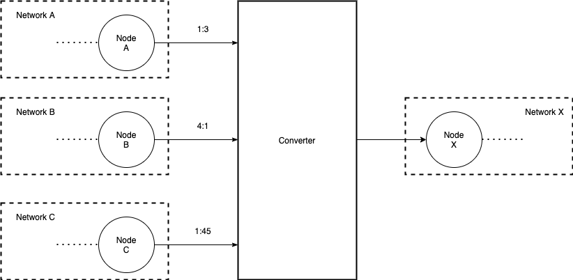
The only difference is how we link node together. If nodes belongs to same network, we use link (or edge) seen before. When nodes belongs to different energies we need to use converter. All things above remains true, we just add now a new element \(V\) converters ont this graph \(G(N, L, V)\) .

Converter can take energy form many nodes in different network. Each converter input has a ratio between output quantity and input quantity. Converter has only one output to only on node.

Variables¶

\(V\) set of converters
\(v \in V\) a converter in the set of converters
\(V^n_\uparrow \subset V\) set of converters to node \(n\)
\(V^n_\downarrow \subset V\) set of converters from node \(n\)
\(\Gamma_v^\uparrow\) flow from converter \(v\).
\(\overline{\Gamma_v^\uparrow}\) max flow from converter \(v\)
\(\gamma_v\) linear cost when \(\Gamma_v^\uparrow\) is used
\(\Gamma_v^\downarrow\) flow(s) to converter. They can have many flows for \(v \in V\), but only one for \(v \in V^n_\downarrow\)
\(\overline{\Gamma_v^\downarrow}\) max flow to converter
\(\alpha^n_v\) ratio conversion for converter \(v\) from node \(n\)

Objective¶

\[\begin{split}\begin{array}{rcl} objective & = & \min{\Omega_{...} + \Omega_{converter}} \\ \Omega_{converter} & = & \sum^V_v {\Gamma_v^\uparrow * \gamma_v} \end{array}\end{split}\]

Constraints¶

Of course Kirschhoff need a little update. Like for storage Warning with naming ! Converter input is a consuming flow for node, converter output is a production flow for node.

\[\begin{array}{rcl} \Pi_{kirschhoff} &:& \forall n \in N &,& [Consuming\ Flow] + \sum^{V^n_\downarrow}_{v}{\Gamma_v^\downarrow} = [Producing\ Flow] + \sum^{V^n_\uparrow}_{v}{\Gamma_v^\uparrow} \end{array}\]

And all these things are bounded :

\[\begin{split}\begin{array}{rcl} \Pi_{Conv\ bound} &:& \left\{\begin{array}{cl} \forall n \in N \\ \forall v \in V^n \end{array} \right. &,& \begin{array}{rcl} 0 &\le& \Gamma_v^\downarrow &\le& \overline{\Gamma_v^\downarrow} \\ 0 &\le& \Gamma_v^\uparrow &\le& \overline{\Gamma_v^\uparrow} \end{array} \end{array}\end{split}\]

Now, we need to fix ratios conversion by a new constraints

\[\begin{split}\begin{array}{rcl} \Pi_{converter} &:& \left\{\begin{array}{cl} \forall n \in N \\ \forall v \in V^n_\downarrow \end{array} \right. &,& \begin{array}{rcl} \Gamma_v^\downarrow * \alpha^n_v &=& \Gamma_v^\uparrow \end{array} \end{array}\end{split}\]