Analyzer¶

For a high abstraction and to be agnostic about technology, Hadar uses objects as glue for optimizer. Objects are cool, but are too complicated to manipulated for data analysis. Analyzer contains tools to help analyzing study and result.

Today, there is only ResultAnalyzer, with two features level:

high level user asks directly to compute global cost and global remain capacity, etc.
low level user build query and get raw data represented inside pandas Dataframe.

Before speaking about this features, let’s see how data are transformed.

Flatten Data¶

As said above, object is nice to encapsulate data and represent it into agnostic form. Objects can be serialized into JSON or something else to be used by another software maybe in another language. But keep object to analyze data is awful.

Python has a very efficient tool for data analysis : pandas. Therefore challenge is to transform object into pandas Dataframe. Solution is to flatten data to fill into table.

Consumption¶

For example with consumption. Data into Study is cost and asked quantity. And in Result it’s cost (same) and given quantity. This tuple (cost, asked, given) is present for each node, each consumption attached on this node, each scenario and each timestep. If we want to flatten data, we need to fill this table

cost	asked	given	node	name	scn	t	network
10	5	5	fr	load	0	0	default
10	7	7	fr	load	0	1	default
10	7	5	fr	load	1	0	default
10	6	6	fr	load	1	1	default
…	…	…	…	…		…	…

It is the purpose of _build_consumption(study: Study, result: Result) -> pd.Dataframe to build this array

Production¶

Production follow the same pattern. However, they don’t have asked and given but available and used quantity. Therefore table looks like

cost	avail	used	node	name	scn	t	network
10	100	21	fr	coal	0	0	default
10	100	36	fr	coal	0	1	default
10	100	12	fr	coal	1	0	default
10	100	81	fr	coal	1	1	default
…	…	…	…	…		…	…

It’s done by _build_production(study: Study, result: Result) -> pd.Dataframe method.

Storage¶

Storage follow the same pattern. Therefore table looks like.

max_capacity	capacity	max_flow_in	flow_in	max_flow_out	flow_out	cost	init_capacity	eff	node	name	scn	t	network
12000	678	400	214	400	0	10	0	.99	fr	cell	0	0	default
12000	892	400	53	400	0	10	0	.99	fr	cell	0	1	default
12000	945	400	0	400	87	10	0	.99	fr	cell	1	0	default
12000	853	400	0	400	0	10	0	.99	fr	cell	1	1	default
…	…	…	…	…	…	…	…	…	…	…		…	…

It’s done by _build_storage(study: Study, result: Result) -> pd.Dataframe method.

Link¶

Link follow the same pattern. Hierarchical structure naming change. There are not node and name but source and destination. Therefore table looks like.

cost	avail	used	src	dest	scn	t	network
10	100	21	fr	uk	0	0	default
10	100	36	fr	uk	0	1	default
10	100	12	fr	uk	1	0	default
10	100	81	fr	uk	1	1	default
…	…	…	…	…			…

It’s done by _build_link(study: Study, result: Result) -> pd.Dataframe method.

Converter¶

Converter follow the same pattern, it just split in two tables. One for source element:

max	ratio	flow	node	name	scn	t	network
100	.4	52	fr	conv	0	0	default
100	.4	87	fr	conv	0	1	default
100	.4	23	fr	conv	1	0	default
100	.4	58	fr	conv	1	1	default
…	…	…	…	…		…	…

It’s done by _build_src_converter(study: Study, result: Result) -> pd.Dataframe method.

And an other for destination element, tables are near identical. Source has special attributes called ratio and destintion has special attribute called cost:

max	cost	flow	node	name	scn	t	network
100	20	52	fr	conv	0	0	default
100	20	87	fr	conv	0	1	default
100	20	23	fr	conv	1	0	default
100	20	58	fr	conv	1	1	default
…	…	…	…	…		…	…

It’s done by _build_dest_converter(study: Study, result: Result) -> pd.Dataframe method.

Low level analysis power with a FluentAPISelector¶

When you observe flat data, there are two kind of data. Content like cost, given, asked and index describes by node, name, scn, t.

Low level API analysis provided by ResultAnalyzer lets user to

Organize index level, for example set time, then scenario, then name, then node.
Filter index, for example just time from 10 to 150, just ‘fr’ node, etc

User can said, I want ‘fr’ node productions for first scenario to 50 until 60 timestep. In this cas ResultAnalyzer will return

		used	cost	avail
t	name	21	fr	uk
50	oil	36	fr	uk
50	coal	12	fr	uk
60 …	oil	81	fr	uk
60 …	…	…	…	…

If first index like node and scenario has only one element, there are removed.

This result can be done by this line of code.

agg = hd.ResultAnalyzer(study, result)
df = agg.network().node('fr').scn(0).time(slice(50, 60)).production()

For analyzer, Fluent API respect these rules:

API flow begin by network()
API flow must contain strictly one of node() , time(), scn() element
API flow must contain only one of element inside link() , production() , consumption()
Except for network(), API has no order. Order is free for user to give hierarchy data.
Therefore above rules, API will always be 5 elements length.

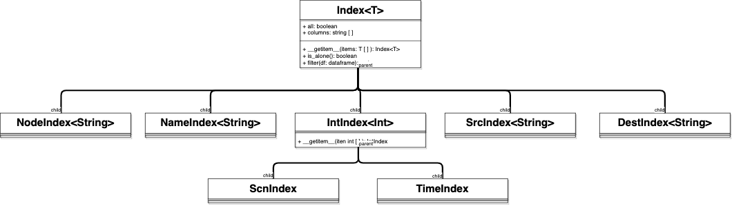
Behind this mechanism, there are Index objects. As you can see directly in the code

...
self.consumption = lambda x=None: self._append(ConsIndex(x))
...
self.time = lambda x=None: self._append(TimeIndex(x))
...

Each kind of index has to inherent from this class. Index object encapsulate column metadata to use and range of filtered elements to keep (accessible by overriding __getitem__ method). Then, Hadar has child classes with good parameters : ConsIndex , ProdIndex , NodeIndex , ScnIndex , TimeIndex , LinkIndex , DestIndex . For example you can find below NodeIndex implementation

class NodeIndex(Index[str]):
    """Index implementation to filter nodes"""
    def __init__(self):
        Index.__init__(self, column='node')

Index instantiation are completely hidden for user. Then, hadar will

check that mandatory indexes are given with _assert_index method.
pivot table to recreate indexing according to filter and sort asked with _pivot method.
remove one-size top-level index with _remove_useless_index_level method.

As you can see, low level analyze provides efficient method to extract data from adequacy study result. However data returned remains a kind of roots and is not ready for business purposes.

High Level Analysis¶

Unlike low level, high level focus on provides ready to use data. Unlike low level, features should be designed one by one for business purpose. Today we have 2 features:

get_cost(self, node: str) -> np.ndarray: method which according to node given returns a matrix (scenario, horizon) shape with summarize cost.
get_balance(self, node: str) -> np.ndarray method which according to node given returns a matrix (scenario, horizon) shape with exchange balance (i.e. sum of exportation minus sum of importation)